10 Data Aggregation and Group Operations
Categorizing a dataset and applying a function to each group, whether an aggregation or transformation, can be a critical component of a data analysis workflow. After loading, merging, and preparing a dataset, you may need to compute group statistics or possibly pivot tables for reporting or visualization purposes. pandas provides a versatile groupby interface, enabling you to slice, dice, and summarize datasets in a natural way.
One reason for the popularity of relational databases and SQL (which stands for “structured query language”) is the ease with which data can be joined, filtered, transformed, and aggregated. However, query languages like SQL impose certain limitations on the kinds of group operations that can be performed. As you will see, with the expressiveness of Python and pandas, we can perform quite complex group operations by expressing them as custom Python functions that manipulate the data associated with each group. In this chapter, you will learn how to:
Split a pandas object into pieces using one or more keys (in the form of functions, arrays, or DataFrame column names)
Calculate group summary statistics, like count, mean, or standard deviation, or a user-defined function
Apply within-group transformations or other manipulations, like normalization, linear regression, rank, or subset selection
Compute pivot tables and cross-tabulations
Perform quantile analysis and other statistical group analyses
Time-based aggregation of time series data, a special use case of groupby, is referred to as resampling in this book and will receive separate treatment in Ch 11: Time Series.
As with the rest of the chapters, we start by importing NumPy and pandas:
In [12]: import numpy as np

In [13]: import pandas as pd
10.1 How to Think About Group Operations
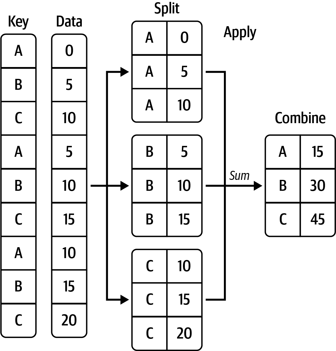
Hadley Wickham, an author of many popular packages for the R programming language, coined the term split-apply-combine for describing group operations. In the first stage of the process, data contained in a pandas object, whether a Series, DataFrame, or otherwise, is split into groups based on one or more keys that you provide. The splitting is performed on a particular axis of an object. For example, a DataFrame can be grouped on its rows (axis="index") or its columns (axis="columns"). Once this is done, a function is applied to each group, producing a new value. Finally, the results of all those function applications are combined into a result object. The form of the resulting object will usually depend on what’s being done to the data. See Figure 10.1 for a mockup of a simple group aggregation.
Each grouping key can take many forms, and the keys do not have to be all of the same type:
A list or array of values that is the same length as the axis being grouped
A value indicating a column name in a DataFrame
A dictionary or Series giving a correspondence between the values on the axis being grouped and the group names
A function to be invoked on the axis index or the individual labels in the index
Note that the latter three methods are shortcuts for producing an array of values to be used to split up the object. Don’t worry if this all seems abstract. Throughout this chapter, I will give many examples of all these methods. To get started, here is a small tabular dataset as a DataFrame:
In [14]: df = pd.DataFrame({"key1" : ["a", "a", None, "b", "b", "a", None],
   ....:                    "key2" : pd.Series([1, 2, 1, 2, 1, None, 1],
   ....:                                       dtype="Int64"),
   ....:                    "data1" : np.random.standard_normal(7),
   ....:                    "data2" : np.random.standard_normal(7)})

In [15]: df
Out[15]:
   key1  key2     data1     data2
0     a     1 -0.204708  0.281746
1     a     2  0.478943  0.769023
2  None     1 -0.519439  1.246435
3     b     2 -0.555730  1.007189
4     b     1  1.965781 -1.296221
5     a  <NA>  1.393406  0.274992
6  None     1  0.092908  0.228913
Suppose you wanted to compute the mean of the data1 column using the labels from key1. There are a number of ways to do this. One is to access data1 and call groupby with the column (a Series) at key1:
In [16]: grouped = df["data1"].groupby(df["key1"])

In [17]: grouped
Out[17]: <pandas.core.groupby.generic.SeriesGroupBy object at 0x17b7913f0>
This grouped variable is now a special "GroupBy" object. It has not actually computed anything yet except for some intermediate data about the group key df["key1"]. The idea is that this object has all of the information needed to then apply some operation to each of the groups. For example, to compute group means we can call the GroupBy’s mean method:
In [18]: grouped.mean()
Out[18]:
key1
a    0.555881
b    0.705025
Name: data1, dtype: float64
Later in Data Aggregation, I'll explain more about what happens when you call .mean(). The important thing here is that the data (a Series) has been aggregated by splitting the data on the group key, producing a new Series that is now indexed by the unique values in the key1 column. The result index has the name "key1" because the DataFrame column df["key1"] did.
If instead we had passed multiple arrays as a list, we'd get something different:
In [19]: means = df["data1"].groupby([df["key1"], df["key2"]]).mean()

In [20]: means
Out[20]:
key1  key2
a     1      -0.204708
      2       0.478943
b     1       1.965781
      2      -0.555730
Name: data1, dtype: float64
Here we grouped the data using two keys, and the resulting Series now has a hierarchical index consisting of the unique pairs of keys observed:
In [21]: means.unstack()
Out[21]:
key2         1         2
key1
a    -0.204708  0.478943
b     1.965781 -0.555730
In this example, the group keys are all Series, though they could be any arrays of the right length:
In [22]: states = np.array(["OH", "CA", "CA", "OH", "OH", "CA", "OH"])

In [23]: years = [2005, 2005, 2006, 2005, 2006, 2005, 2006]

In [24]: df["data1"].groupby([states, years]).mean()
Out[24]:
CA  2005    0.936175
    2006   -0.519439
OH  2005   -0.380219
    2006    1.029344
Name: data1, dtype: float64
Frequently, the grouping information is found in the same DataFrame as the data you want to work on. In that case, you can pass column names (whether those are strings, numbers, or other Python objects) as the group keys:
In [25]: df.groupby("key1").mean()
Out[25]:
      key2     data1     data2
key1
a      1.5  0.555881  0.441920
b      1.5  0.705025 -0.144516

In [26]: df.groupby("key2").mean(numeric_only=True)
Out[26]:
         data1     data2
key2
1     0.333636  0.115218
2    -0.038393  0.888106

In [27]: df.groupby(["key1", "key2"]).mean()
Out[27]:
              data1     data2
key1 key2
a    1    -0.204708  0.281746
     2     0.478943  0.769023
b    1     1.965781 -1.296221
     2    -0.555730  1.007189
You may notice that in the second case, it is necessary to pass numeric_only=True because the key1 column is not numeric and thus cannot be aggregated with mean().
Regardless of the objective in using groupby, a generally useful GroupBy method is size, which returns a Series containing group sizes:
In [28]: df.groupby(["key1", "key2"]).size()
Out[28]:
key1  key2
a     1       1
      2       1
b     1       1
      2       1
dtype: int64
Note that any missing values in a group key are excluded from the result by default. This behavior can be disabled by passing dropna=False to groupby:
In [29]: df.groupby("key1", dropna=False).size()
Out[29]:
key1
a      3
b      2
NaN    2
dtype: int64

In [30]: df.groupby(["key1", "key2"], dropna=False).size()
Out[30]:
key1  key2
a     1       1
      2       1
      <NA>    1
b     1       1
      2       1
NaN   1       2
dtype: int64
A group function similar in spirit to size is count, which computes the number of nonnull values in each group:
In [31]: df.groupby("key1").count()
Out[31]:
      key2  data1  data2
key1
a        2      3      3
b        2      2      2
Iterating over Groups
The object returned by groupby supports iteration, generating a sequence of 2-tuples containing the group name along with the chunk of data. Consider the following:
In [32]: for name, group in df.groupby("key1"):
   ....:     print(name)
   ....:     print(group)
   ....:
a
  key1  key2     data1     data2
0    a     1 -0.204708  0.281746
1    a     2  0.478943  0.769023
5    a  <NA>  1.393406  0.274992
b
  key1  key2     data1     data2
3    b     2 -0.555730  1.007189
4    b     1  1.965781 -1.296221
In the case of multiple keys, the first element in the tuple will be a tuple of key values:
In [33]: for (k1, k2), group in df.groupby(["key1", "key2"]):
   ....:     print((k1, k2))
   ....:     print(group)
   ....:
('a', 1)
  key1  key2     data1     data2
0    a     1 -0.204708  0.281746
('a', 2)
  key1  key2     data1     data2
1    a     2  0.478943  0.769023
('b', 1)
  key1  key2     data1     data2
4    b     1  1.965781 -1.296221
('b', 2)
  key1  key2    data1     data2
3    b     2 -0.55573  1.007189
Of course, you can choose to do whatever you want with the pieces of data. A recipe you may find useful is computing a dictionary of the data pieces as a one-liner:
In [34]: pieces = {name: group for name, group in df.groupby("key1")}

In [35]: pieces["b"]
Out[35]:
  key1  key2     data1     data2
3    b     2 -0.555730  1.007189
4    b     1  1.965781 -1.296221
By default groupby groups on axis="index", but you can group on any of the other axes. For example, we could group the columns of our example df here by whether they start with "key" or "data":
In [36]: grouped = df.groupby({"key1": "key", "key2": "key",
   ....:                       "data1": "data", "data2": "data"}, axis="columns")
We can print out the groups like so:
In [37]: for group_key, group_values in grouped:
   ....:     print(group_key)
   ....:     print(group_values)
   ....:
data
      data1     data2
0 -0.204708  0.281746
1  0.478943  0.769023
2 -0.519439  1.246435
3 -0.555730  1.007189
4  1.965781 -1.296221
5  1.393406  0.274992
6  0.092908  0.228913
key
   key1  key2
0     a     1
1     a     2
2  None     1
3     b     2
4     b     1
5     a  <NA>
6  None     1
Selecting a Column or Subset of Columns
Indexing a GroupBy object created from a DataFrame with a column name or array of column names has the effect of column subsetting for aggregation. This means that:
df.groupby("key1")["data1"]
df.groupby("key1")[["data2"]]
are conveniences for:
df["data1"].groupby(df["key1"])
df[["data2"]].groupby(df["key1"])
Especially for large datasets, it may be desirable to aggregate only a few columns. For example, in the preceding dataset, to compute the means for just the data2 column and get the result as a DataFrame, we could write:
In [38]: df.groupby(["key1", "key2"])[["data2"]].mean()
Out[38]:
              data2
key1 key2
a    1     0.281746
     2     0.769023
b    1    -1.296221
     2     1.007189
The object returned by this indexing operation is a grouped DataFrame if a list or array is passed, or a grouped Series if only a single column name is passed as a scalar:
In [39]: s_grouped = df.groupby(["key1", "key2"])["data2"]

In [40]: s_grouped
Out[40]: <pandas.core.groupby.generic.SeriesGroupBy object at 0x17b8356c0>

In [41]: s_grouped.mean()
Out[41]:
key1  key2
a     1       0.281746
      2       0.769023
b     1      -1.296221
      2       1.007189
Name: data2, dtype: float64
Grouping with Dictionaries and Series
Grouping information may exist in a form other than an array. Let’s consider another example DataFrame:
In [42]: people = pd.DataFrame(np.random.standard_normal((5, 5)),
   ....:                       columns=["a", "b", "c", "d", "e"],
   ....:                       index=["Joe", "Steve", "Wanda", "Jill", "Trey"])

In [43]: people.iloc[2:3, [1, 2]] = np.nan # Add a few NA values

In [44]: people
Out[44]:
              a         b         c         d         e
Joe    1.352917  0.886429 -2.001637 -0.371843  1.669025
Steve -0.438570 -0.539741  0.476985  3.248944 -1.021228
Wanda -0.577087       NaN       NaN  0.523772  0.000940
Jill   1.343810 -0.713544 -0.831154 -2.370232 -1.860761
Trey  -0.860757  0.560145 -1.265934  0.119827 -1.063512
Now, suppose I have a group correspondence for the columns and want to sum the columns by group:
In [45]: mapping = {"a": "red", "b": "red", "c": "blue",
   ....:            "d": "blue", "e": "red", "f" : "orange"}
Now, you could construct an array from this dictionary to pass to groupby, but instead we can just pass the dictionary (I included the key "f" to highlight that unused grouping keys are OK):
In [46]: by_column = people.groupby(mapping, axis="columns")

In [47]: by_column.sum()
Out[47]:
           blue       red
Joe   -2.373480  3.908371
Steve  3.725929 -1.999539
Wanda  0.523772 -0.576147
Jill  -3.201385 -1.230495
Trey  -1.146107 -1.364125
The same functionality holds for Series, which can be viewed as a fixed-size mapping:
In [48]: map_series = pd.Series(mapping)

In [49]: map_series
Out[49]:
a       red
b       red
c      blue
d      blue
e       red
f    orange
dtype: object

In [50]: people.groupby(map_series, axis="columns").count()
Out[50]:
       blue  red
Joe       2    3
Steve     2    3
Wanda     1    2
Jill      2    3
Trey      2    3
Grouping with Functions
Using Python functions is a more generic way of defining a group mapping compared with a dictionary or Series. Any function passed as a group key will be called once per index value (or once per column value if using axis="columns"), with the return values being used as the group names. More concretely, consider the example DataFrame from the previous section, which has people’s first names as index values. Suppose you wanted to group by name length. While you could compute an array of string lengths, it's simpler to just pass the len function:
In [51]: people.groupby(len).sum()
Out[51]:
          a         b         c         d         e
3  1.352917  0.886429 -2.001637 -0.371843  1.669025
4  0.483052 -0.153399 -2.097088 -2.250405 -2.924273
5 -1.015657 -0.539741  0.476985  3.772716 -1.020287
Mixing functions with arrays, dictionaries, or Series is not a problem, as everything gets converted to arrays internally:
In [52]: key_list = ["one", "one", "one", "two", "two"]

In [53]: people.groupby([len, key_list]).min()
Out[53]:
              a         b         c         d         e
3 one  1.352917  0.886429 -2.001637 -0.371843  1.669025
4 two -0.860757 -0.713544 -1.265934 -2.370232 -1.860761
5 one -0.577087 -0.539741  0.476985  0.523772 -1.021228
Grouping by Index Levels
A final convenience for hierarchically indexed datasets is the ability to aggregate using one of the levels of an axis index. Let's look at an example:
In [54]: columns = pd.MultiIndex.from_arrays([["US", "US", "US", "JP", "JP"],
   ....:                                     [1, 3, 5, 1, 3]],
   ....:                                     names=["cty", "tenor"])

In [55]: hier_df = pd.DataFrame(np.random.standard_normal((4, 5)), columns=column
s)

In [56]: hier_df
Out[56]:
cty          US                            JP
tenor         1         3         5         1         3
0      0.332883 -2.359419 -0.199543 -1.541996 -0.970736
1     -1.307030  0.286350  0.377984 -0.753887  0.331286
2      1.349742  0.069877  0.246674 -0.011862  1.004812
3      1.327195 -0.919262 -1.549106  0.022185  0.758363
To group by level, pass the level number or name using the level keyword:
In [57]: hier_df.groupby(level="cty", axis="columns").count()
Out[57]:
cty  JP  US
0     2   3
1     2   3
2     2   3
3     2   3
10.2 Data Aggregation
Aggregations refer to any data transformation that produces scalar values from arrays. The preceding examples have used several of them, including mean, count, min, and sum. You may wonder what is going on when you invoke mean() on a GroupBy object. Many common aggregations, such as those found in Table 10.1, have optimized implementations. However, you are not limited to only this set of methods.
| Function name | Description |
|---|---|
any, all |
Return True if any (one or more values) or all non-NA values are "truthy" |
count |
Number of non-NA values |
cummin, cummax |
Cumulative minimum and maximum of non-NA values |
cumsum |
Cumulative sum of non-NA values |
cumprod |
Cumulative product of non-NA values |
first, last |
First and last non-NA values |
mean |
Mean of non-NA values |
median |
Arithmetic median of non-NA values |
min, max |
Minimum and maximum of non-NA values |
nth |
Retrieve value that would appear at position n with the data in sorted order |
ohlc |
Compute four "open-high-low-close" statistics for time series-like data |
prod |
Product of non-NA values |
quantile |
Compute sample quantile |
rank |
Ordinal ranks of non-NA values, like calling Series.rank |
size |
Compute group sizes, returning result as a Series |
sum |
Sum of non-NA values |
std, var |
Sample standard deviation and variance |
You can use aggregations of your own devising and additionally call any method that is also defined on the object being grouped. For example, the nsmallest Series method selects the smallest requested number of values from the data. While nsmallest is not explicitly implemented for GroupBy, we can still use it with a nonoptimized implementation. Internally, GroupBy slices up the Series, calls piece.nsmallest(n) for each piece, and then assembles those results into the result object:
In [58]: df
Out[58]:
   key1  key2     data1     data2
0     a     1 -0.204708  0.281746
1     a     2  0.478943  0.769023
2  None     1 -0.519439  1.246435
3     b     2 -0.555730  1.007189
4     b     1  1.965781 -1.296221
5     a  <NA>  1.393406  0.274992
6  None     1  0.092908  0.228913

In [59]: grouped = df.groupby("key1")

In [60]: grouped["data1"].nsmallest(2)
Out[60]:
key1
a     0   -0.204708
      1    0.478943
b     3   -0.555730
      4    1.965781
Name: data1, dtype: float64
To use your own aggregation functions, pass any function that aggregates an array to the aggregate method or its short alias agg:
In [61]: def peak_to_peak(arr):
   ....:     return arr.max() - arr.min()

In [62]: grouped.agg(peak_to_peak)
Out[62]:
      key2     data1     data2
key1
a        1  1.598113  0.494031
b        1  2.521511  2.303410
You may notice that some methods, like describe, also work, even though they are not aggregations, strictly speaking:
In [63]: grouped.describe()
Out[63]:
      key2                                           data1            ...
     count mean       std  min   25%  50%   75%  max count      mean  ...
key1                                                                  ...
a      2.0  1.5  0.707107  1.0  1.25  1.5  1.75  2.0   3.0  0.555881  ...  \
b      2.0  1.5  0.707107  1.0  1.25  1.5  1.75  2.0   2.0  0.705025  ...
                         data2
           75%       max count      mean       std       min       25%
key1
a     0.936175  1.393406   3.0  0.441920  0.283299  0.274992  0.278369  \
b     1.335403  1.965781   2.0 -0.144516  1.628757 -1.296221 -0.720368

           50%       75%       max
key1
a     0.281746  0.525384  0.769023
b    -0.144516  0.431337  1.007189
[2 rows x 24 columns]
I will explain in more detail what has happened here in Apply: General split-apply-combine.
Custom aggregation functions are generally much slower than the optimized functions found in Table 10.1. This is because there is some extra overhead (function calls, data rearrangement) in constructing the intermediate group data chunks.
Column-Wise and Multiple Function Application
Let's return to the tipping dataset used in the last chapter. After loading it with pandas.read_csv, we add a tipping percentage column:
In [64]: tips = pd.read_csv("examples/tips.csv")

In [65]: tips.head()
Out[65]:
   total_bill   tip smoker  day    time  size
0       16.99  1.01     No  Sun  Dinner     2
1       10.34  1.66     No  Sun  Dinner     3
2       21.01  3.50     No  Sun  Dinner     3
3       23.68  3.31     No  Sun  Dinner     2
4       24.59  3.61     No  Sun  Dinner     4
Now I will add a tip_pct column with the tip percentage of the total bill:
In [66]: tips["tip_pct"] = tips["tip"] / tips["total_bill"]

In [67]: tips.head()
Out[67]:
   total_bill   tip smoker  day    time  size   tip_pct
0       16.99  1.01     No  Sun  Dinner     2  0.059447
1       10.34  1.66     No  Sun  Dinner     3  0.160542
2       21.01  3.50     No  Sun  Dinner     3  0.166587
3       23.68  3.31     No  Sun  Dinner     2  0.139780
4       24.59  3.61     No  Sun  Dinner     4  0.146808
As you’ve already seen, aggregating a Series or all of the columns of a DataFrame is a matter of using aggregate (or agg) with the desired function or calling a method like mean or std. However, you may want to aggregate using a different function, depending on the column, or multiple functions at once. Fortunately, this is possible to do, which I’ll illustrate through a number of examples. First, I’ll group the tips by day and smoker:
In [68]: grouped = tips.groupby(["day", "smoker"])Note that for descriptive statistics like those in Table 10.1, you can pass the name of the function as a string:
In [69]: grouped_pct = grouped["tip_pct"]

In [70]: grouped_pct.agg("mean")
Out[70]:
day   smoker
Fri   No        0.151650
      Yes       0.174783
Sat   No        0.158048
      Yes       0.147906
Sun   No        0.160113
      Yes       0.187250
Thur  No        0.160298
      Yes       0.163863
Name: tip_pct, dtype: float64
If you pass a list of functions or function names instead, you get back a DataFrame with column names taken from the functions:
In [71]: grouped_pct.agg(["mean", "std", peak_to_peak])
Out[71]:
                 mean       std  peak_to_peak
day  smoker
Fri  No      0.151650  0.028123      0.067349
     Yes     0.174783  0.051293      0.159925
Sat  No      0.158048  0.039767      0.235193
     Yes     0.147906  0.061375      0.290095
Sun  No      0.160113  0.042347      0.193226
     Yes     0.187250  0.154134      0.644685
Thur No      0.160298  0.038774      0.193350
     Yes     0.163863  0.039389      0.151240
Here we passed a list of aggregation functions to agg to evaluate independently on the data groups.
You don’t need to accept the names that GroupBy gives to the columns; notably, lambda functions have the name "<lambda>", which makes them hard to identify (you can see for yourself by looking at a function’s __name__ attribute). Thus, if you pass a list of (name, function) tuples, the first element of each tuple will be used as the DataFrame column names (you can think of a list of 2-tuples as an ordered mapping):
In [72]: grouped_pct.agg([("average", "mean"), ("stdev", np.std)])
Out[72]:
              average     stdev
day  smoker
Fri  No      0.151650  0.028123
     Yes     0.174783  0.051293
Sat  No      0.158048  0.039767
     Yes     0.147906  0.061375
Sun  No      0.160113  0.042347
     Yes     0.187250  0.154134
Thur No      0.160298  0.038774
     Yes     0.163863  0.039389
With a DataFrame you have more options, as you can specify a list of functions to apply to all of the columns or different functions per column. To start, suppose we wanted to compute the same three statistics for the tip_pct and total_bill columns:
In [73]: functions = ["count", "mean", "max"]

In [74]: result = grouped[["tip_pct", "total_bill"]].agg(functions)

In [75]: result
Out[75]:
            tip_pct                     total_bill
              count      mean       max      count       mean    max
day  smoker
Fri  No           4  0.151650  0.187735          4  18.420000  22.75
     Yes         15  0.174783  0.263480         15  16.813333  40.17
Sat  No          45  0.158048  0.291990         45  19.661778  48.33
     Yes         42  0.147906  0.325733         42  21.276667  50.81
Sun  No          57  0.160113  0.252672         57  20.506667  48.17
     Yes         19  0.187250  0.710345         19  24.120000  45.35
Thur No          45  0.160298  0.266312         45  17.113111  41.19
     Yes         17  0.163863  0.241255         17  19.190588  43.11
As you can see, the resulting DataFrame has hierarchical columns, the same as you would get aggregating each column separately and using concat to glue the results together using the column names as the keys argument:
In [76]: result["tip_pct"]
Out[76]:
             count      mean       max
day  smoker
Fri  No          4  0.151650  0.187735
     Yes        15  0.174783  0.263480
Sat  No         45  0.158048  0.291990
     Yes        42  0.147906  0.325733
Sun  No         57  0.160113  0.252672
     Yes        19  0.187250  0.710345
Thur No         45  0.160298  0.266312
     Yes        17  0.163863  0.241255
As before, a list of tuples with custom names can be passed:
In [77]: ftuples = [("Average", "mean"), ("Variance", np.var)]

In [78]: grouped[["tip_pct", "total_bill"]].agg(ftuples)
Out[78]:
              tip_pct           total_bill
              Average  Variance    Average    Variance
day  smoker
Fri  No      0.151650  0.000791  18.420000   25.596333
     Yes     0.174783  0.002631  16.813333   82.562438
Sat  No      0.158048  0.001581  19.661778   79.908965
     Yes     0.147906  0.003767  21.276667  101.387535
Sun  No      0.160113  0.001793  20.506667   66.099980
     Yes     0.187250  0.023757  24.120000  109.046044
Thur No      0.160298  0.001503  17.113111   59.625081
     Yes     0.163863  0.001551  19.190588   69.808518
Now, suppose you wanted to apply potentially different functions to one or more of the columns. To do this, pass a dictionary to agg that contains a mapping of column names to any of the function specifications listed so far:
In [79]: grouped.agg({"tip" : np.max, "size" : "sum"})
Out[79]:
               tip  size
day  smoker
Fri  No       3.50     9
     Yes      4.73    31
Sat  No       9.00   115
     Yes     10.00   104
Sun  No       6.00   167
     Yes      6.50    49
Thur No       6.70   112
     Yes      5.00    40

In [80]: grouped.agg({"tip_pct" : ["min", "max", "mean", "std"],
   ....:              "size" : "sum"})
Out[80]:
              tip_pct                               size
                  min       max      mean       std  sum
day  smoker
Fri  No      0.120385  0.187735  0.151650  0.028123    9
     Yes     0.103555  0.263480  0.174783  0.051293   31
Sat  No      0.056797  0.291990  0.158048  0.039767  115
     Yes     0.035638  0.325733  0.147906  0.061375  104
Sun  No      0.059447  0.252672  0.160113  0.042347  167
     Yes     0.065660  0.710345  0.187250  0.154134   49
Thur No      0.072961  0.266312  0.160298  0.038774  112
     Yes     0.090014  0.241255  0.163863  0.039389   40
A DataFrame will have hierarchical columns only if multiple functions are applied to at least one column.
Returning Aggregated Data Without Row Indexes
In all of the examples up until now, the aggregated data comes back with an index, potentially hierarchical, composed from the unique group key combinations. Since this isn’t always desirable, you can disable this behavior in most cases by passing as_index=False to groupby:
In [81]: grouped = tips.groupby(["day", "smoker"], as_index=False)

In [82]: grouped.mean(numeric_only=True)
Out[82]:
    day smoker  total_bill       tip      size   tip_pct
0   Fri     No   18.420000  2.812500  2.250000  0.151650
1   Fri    Yes   16.813333  2.714000  2.066667  0.174783
2   Sat     No   19.661778  3.102889  2.555556  0.158048
3   Sat    Yes   21.276667  2.875476  2.476190  0.147906
4   Sun     No   20.506667  3.167895  2.929825  0.160113
5   Sun    Yes   24.120000  3.516842  2.578947  0.187250
6  Thur     No   17.113111  2.673778  2.488889  0.160298
7  Thur    Yes   19.190588  3.030000  2.352941  0.163863
Of course, it’s always possible to obtain the result in this format by calling reset_index on the result. Using the as_index=False argument avoids some unnecessary computations.
10.3 Apply: General split-apply-combine
The most general-purpose GroupBy method is apply, which is the subject of this section. apply splits the object being manipulated into pieces, invokes the passed function on each piece, and then attempts to concatenate the pieces.
Returning to the tipping dataset from before, suppose you wanted to select the top five tip_pct values by group. First, write a function that selects the rows with the largest values in a particular column:
In [83]: def top(df, n=5, column="tip_pct"):
   ....:     return df.sort_values(column, ascending=False)[:n]

In [84]: top(tips, n=6)
Out[84]:
     total_bill   tip smoker  day    time  size   tip_pct
172        7.25  5.15    Yes  Sun  Dinner     2  0.710345
178        9.60  4.00    Yes  Sun  Dinner     2  0.416667
67         3.07  1.00    Yes  Sat  Dinner     1  0.325733
232       11.61  3.39     No  Sat  Dinner     2  0.291990
183       23.17  6.50    Yes  Sun  Dinner     4  0.280535
109       14.31  4.00    Yes  Sat  Dinner     2  0.279525
Now, if we group by smoker, say, and call apply with this function, we get the following:
In [85]: tips.groupby("smoker").apply(top)
Out[85]:
            total_bill   tip smoker   day    time  size   tip_pct
smoker
No     232       11.61  3.39     No   Sat  Dinner     2  0.291990
       149        7.51  2.00     No  Thur   Lunch     2  0.266312
       51        10.29  2.60     No   Sun  Dinner     2  0.252672
       185       20.69  5.00     No   Sun  Dinner     5  0.241663
       88        24.71  5.85     No  Thur   Lunch     2  0.236746
Yes    172        7.25  5.15    Yes   Sun  Dinner     2  0.710345
       178        9.60  4.00    Yes   Sun  Dinner     2  0.416667
       67         3.07  1.00    Yes   Sat  Dinner     1  0.325733
       183       23.17  6.50    Yes   Sun  Dinner     4  0.280535
       109       14.31  4.00    Yes   Sat  Dinner     2  0.279525
What has happened here? First, the tips DataFrame is split into groups based on the value of smoker. Then the top function is called on each group, and the results of each function call are glued together using pandas.concat, labeling the pieces with the group names. The result therefore has a hierarchical index with an inner level that contains index values from the original DataFrame.
If you pass a function to apply that takes other arguments or keywords, you can pass these after the function:
In [86]: tips.groupby(["smoker", "day"]).apply(top, n=1, column="total_bill")
Out[86]:
                 total_bill    tip smoker   day    time  size   tip_pct
smoker day
No     Fri  94        22.75   3.25     No   Fri  Dinner     2  0.142857
       Sat  212       48.33   9.00     No   Sat  Dinner     4  0.186220
       Sun  156       48.17   5.00     No   Sun  Dinner     6  0.103799
       Thur 142       41.19   5.00     No  Thur   Lunch     5  0.121389
Yes    Fri  95        40.17   4.73    Yes   Fri  Dinner     4  0.117750
       Sat  170       50.81  10.00    Yes   Sat  Dinner     3  0.196812
       Sun  182       45.35   3.50    Yes   Sun  Dinner     3  0.077178
       Thur 197       43.11   5.00    Yes  Thur   Lunch     4  0.115982
Beyond these basic usage mechanics, getting the most out of apply may require some creativity. What occurs inside the function passed is up to you; it must either return a pandas object or a scalar value. The rest of this chapter will consist mainly of examples showing you how to solve various problems using groupby.
For example, you may recall that I earlier called describe on a GroupBy object:
In [87]: result = tips.groupby("smoker")["tip_pct"].describe()

In [88]: result
Out[88]:
        count      mean       std       min       25%       50%       75%
smoker
No      151.0  0.159328  0.039910  0.056797  0.136906  0.155625  0.185014  \
Yes      93.0  0.163196  0.085119  0.035638  0.106771  0.153846  0.195059
             max
smoker
No      0.291990
Yes     0.710345

In [89]: result.unstack("smoker")
Out[89]:
       smoker
count  No        151.000000
       Yes        93.000000
mean   No          0.159328
       Yes         0.163196
std    No          0.039910
       Yes         0.085119
min    No          0.056797
       Yes         0.035638
25%    No          0.136906
       Yes         0.106771
50%    No          0.155625
       Yes         0.153846
75%    No          0.185014
       Yes         0.195059
max    No          0.291990
       Yes         0.710345
dtype: float64
Inside GroupBy, when you invoke a method like describe, it is actually just a shortcut for:
def f(group):
    return group.describe()

grouped.apply(f)
Suppressing the Group Keys
In the preceding examples, you see that the resulting object has a hierarchical index formed from the group keys, along with the indexes of each piece of the original object. You can disable this by passing group_keys=False to groupby:
In [90]: tips.groupby("smoker", group_keys=False).apply(top)
Out[90]:
     total_bill   tip smoker   day    time  size   tip_pct
232       11.61  3.39     No   Sat  Dinner     2  0.291990
149        7.51  2.00     No  Thur   Lunch     2  0.266312
51        10.29  2.60     No   Sun  Dinner     2  0.252672
185       20.69  5.00     No   Sun  Dinner     5  0.241663
88        24.71  5.85     No  Thur   Lunch     2  0.236746
172        7.25  5.15    Yes   Sun  Dinner     2  0.710345
178        9.60  4.00    Yes   Sun  Dinner     2  0.416667
67         3.07  1.00    Yes   Sat  Dinner     1  0.325733
183       23.17  6.50    Yes   Sun  Dinner     4  0.280535
109       14.31  4.00    Yes   Sat  Dinner     2  0.279525
Quantile and Bucket Analysis
As you may recall from Ch 8: Data Wrangling: Join, Combine, and Reshape, pandas has some tools, in particular pandas.cut and pandas.qcut, for slicing data up into buckets with bins of your choosing, or by sample quantiles. Combining these functions with groupby makes it convenient to perform bucket or quantile analysis on a dataset. Consider a simple random dataset and an equal-length bucket categorization using pandas.cut:
In [91]: frame = pd.DataFrame({"data1": np.random.standard_normal(1000),
   ....:                       "data2": np.random.standard_normal(1000)})

In [92]: frame.head()
Out[92]:
      data1     data2
0 -0.660524 -0.612905
1  0.862580  0.316447
2 -0.010032  0.838295
3  0.050009 -1.034423
4  0.670216  0.434304

In [93]: quartiles = pd.cut(frame["data1"], 4)

In [94]: quartiles.head(10)
Out[94]:
0     (-1.23, 0.489]
1     (0.489, 2.208]
2     (-1.23, 0.489]
3     (-1.23, 0.489]
4     (0.489, 2.208]
5     (0.489, 2.208]
6     (-1.23, 0.489]
7     (-1.23, 0.489]
8    (-2.956, -1.23]
9     (-1.23, 0.489]
Name: data1, dtype: category
Categories (4, interval[float64, right]): [(-2.956, -1.23] < (-1.23, 0.489] < (0.
489, 2.208] <
                                           (2.208, 3.928]]
The Categorical object returned by cut can be passed directly to groupby. So we could compute a set of group statistics for the quartiles, like so:
In [95]: def get_stats(group):
   ....:     return pd.DataFrame(
   ....:         {"min": group.min(), "max": group.max(),
   ....:         "count": group.count(), "mean": group.mean()}
   ....:     )

In [96]: grouped = frame.groupby(quartiles)

In [97]: grouped.apply(get_stats)
Out[97]:
                            min       max  count      mean
data1
(-2.956, -1.23] data1 -2.949343 -1.230179     94 -1.658818
                data2 -3.399312  1.670835     94 -0.033333
(-1.23, 0.489]  data1 -1.228918  0.488675    598 -0.329524
                data2 -2.989741  3.260383    598 -0.002622
(0.489, 2.208]  data1  0.489965  2.200997    298  1.065727
                data2 -3.745356  2.954439    298  0.078249
(2.208, 3.928]  data1  2.212303  3.927528     10  2.644253
                data2 -1.929776  1.765640     10  0.024750
Keep in mind the same result could have been computed more simply with:
In [98]: grouped.agg(["min", "max", "count", "mean"])
Out[98]:
                    data1                               data2
                      min       max count      mean       min       max count
data1
(-2.956, -1.23] -2.949343 -1.230179    94 -1.658818 -3.399312  1.670835    94  \
(-1.23, 0.489]  -1.228918  0.488675   598 -0.329524 -2.989741  3.260383   598
(0.489, 2.208]   0.489965  2.200997   298  1.065727 -3.745356  2.954439   298
(2.208, 3.928]   2.212303  3.927528    10  2.644253 -1.929776  1.765640    10

                     mean
data1
(-2.956, -1.23] -0.033333
(-1.23, 0.489]  -0.002622
(0.489, 2.208]   0.078249
(2.208, 3.928]   0.024750
These were equal-length buckets; to compute equal-size buckets based on sample quantiles, use pandas.qcut. We can pass 4 as the number of bucket compute sample quartiles, and pass labels=False to obtain just the quartile indices instead of intervals:
In [99]: quartiles_samp = pd.qcut(frame["data1"], 4, labels=False)

In [100]: quartiles_samp.head()
Out[100]:
0    1
1    3
2    2
3    2
4    3
Name: data1, dtype: int64

In [101]: grouped = frame.groupby(quartiles_samp)

In [102]: grouped.apply(get_stats)
Out[102]:
                  min       max  count      mean
data1
0     data1 -2.949343 -0.685484    250 -1.212173
      data2 -3.399312  2.628441    250 -0.027045
1     data1 -0.683066 -0.030280    250 -0.368334
      data2 -2.630247  3.260383    250 -0.027845
2     data1 -0.027734  0.618965    250  0.295812
      data2 -3.056990  2.458842    250  0.014450
3     data1  0.623587  3.927528    250  1.248875
      data2 -3.745356  2.954439    250  0.115899
Example: Filling Missing Values with Group-Specific Values
When cleaning up missing data, in some cases you will remove data observations using dropna, but in others you may want to fill in the null (NA) values using a fixed value or some value derived from the data. fillna is the right tool to use; for example, here I fill in the null values with the mean:
In [103]: s = pd.Series(np.random.standard_normal(6))

In [104]: s[::2] = np.nan

In [105]: s
Out[105]:
0         NaN
1    0.227290
2         NaN
3   -2.153545
4         NaN
5   -0.375842
dtype: float64

In [106]: s.fillna(s.mean())
Out[106]:
0   -0.767366
1    0.227290
2   -0.767366
3   -2.153545
4   -0.767366
5   -0.375842
dtype: float64
Suppose you need the fill value to vary by group. One way to do this is to group the data and use apply with a function that calls fillna on each data chunk. Here is some sample data on US states divided into eastern and western regions:
In [107]: states = ["Ohio", "New York", "Vermont", "Florida",
   .....:           "Oregon", "Nevada", "California", "Idaho"]

In [108]: group_key = ["East", "East", "East", "East",
   .....:              "West", "West", "West", "West"]

In [109]: data = pd.Series(np.random.standard_normal(8), index=states)

In [110]: data
Out[110]:
Ohio          0.329939
New York      0.981994
Vermont       1.105913
Florida      -1.613716
Oregon        1.561587
Nevada        0.406510
California    0.359244
Idaho        -0.614436
dtype: float64
Let's set some values in the data to be missing:
In [111]: data[["Vermont", "Nevada", "Idaho"]] = np.nan

In [112]: data
Out[112]:
Ohio          0.329939
New York      0.981994
Vermont            NaN
Florida      -1.613716
Oregon        1.561587
Nevada             NaN
California    0.359244
Idaho              NaN
dtype: float64

In [113]: data.groupby(group_key).size()
Out[113]:
East    4
West    4
dtype: int64

In [114]: data.groupby(group_key).count()
Out[114]:
East    3
West    2
dtype: int64

In [115]: data.groupby(group_key).mean()
Out[115]:
East   -0.100594
West    0.960416
dtype: float64
We can fill the NA values using the group means, like so:
In [116]: def fill_mean(group):
   .....:     return group.fillna(group.mean())

In [117]: data.groupby(group_key).apply(fill_mean)
Out[117]:
East  Ohio          0.329939
      New York      0.981994
      Vermont      -0.100594
      Florida      -1.613716
West  Oregon        1.561587
      Nevada        0.960416
      California    0.359244
      Idaho         0.960416
dtype: float64
In another case, you might have predefined fill values in your code that vary by group. Since the groups have a name attribute set internally, we can use that:
In [118]: fill_values = {"East": 0.5, "West": -1}

In [119]: def fill_func(group):
   .....:     return group.fillna(fill_values[group.name])

In [120]: data.groupby(group_key).apply(fill_func)
Out[120]:
East  Ohio          0.329939
      New York      0.981994
      Vermont       0.500000
      Florida      -1.613716
West  Oregon        1.561587
      Nevada       -1.000000
      California    0.359244
      Idaho        -1.000000
dtype: float64
Example: Random Sampling and Permutation
Suppose you wanted to draw a random sample (with or without replacement) from a large dataset for Monte Carlo simulation purposes or some other application. There are a number of ways to perform the “draws”; here we use the sample method for Series.
To demonstrate, here’s a way to construct a deck of English-style playing cards:
suits = ["H", "S", "C", "D"]  # Hearts, Spades, Clubs, Diamonds
card_val = (list(range(1, 11)) + [10] * 3) * 4
base_names = ["A"] + list(range(2, 11)) + ["J", "K", "Q"]
cards = []
for suit in suits:
    cards.extend(str(num) + suit for num in base_names)

deck = pd.Series(card_val, index=cards)
Now we have a Series of length 52 whose index contains card names, and values are the ones used in blackjack and other games (to keep things simple, I let the ace "A" be 1):
In [122]: deck.head(13)
Out[122]:
AH      1
2H      2
3H      3
4H      4
5H      5
6H      6
7H      7
8H      8
9H      9
10H    10
JH     10
KH     10
QH     10
dtype: int64
Now, based on what I said before, drawing a hand of five cards from the deck could be written as:
In [123]: def draw(deck, n=5):
   .....:     return deck.sample(n)

In [124]: draw(deck)
Out[124]:
4D     4
QH    10
8S     8
7D     7
9C     9
dtype: int64
Suppose you wanted two random cards from each suit. Because the suit is the last character of each card name, we can group based on this and use apply:
In [125]: def get_suit(card):
   .....:     # last letter is suit
   .....:     return card[-1]

In [126]: deck.groupby(get_suit).apply(draw, n=2)
Out[126]:
C  6C     6
   KC    10
D  7D     7
   3D     3
H  7H     7
   9H     9
S  2S     2
   QS    10
dtype: int64
Alternatively, we could pass group_keys=False to drop the outer suit index, leaving in just the selected cards:
In [127]: deck.groupby(get_suit, group_keys=False).apply(draw, n=2)
Out[127]:
AC      1
3C      3
5D      5
4D      4
10H    10
7H      7
QS     10
7S      7
dtype: int64
Example: Group Weighted Average and Correlation
Under the split-apply-combine paradigm of groupby, operations between columns in a DataFrame or two Series, such as a group weighted average, are possible. As an example, take this dataset containing group keys, values, and some weights:
In [128]: df = pd.DataFrame({"category": ["a", "a", "a", "a",
   .....:                                 "b", "b", "b", "b"],
   .....:                    "data": np.random.standard_normal(8),
   .....:                    "weights": np.random.uniform(size=8)})

In [129]: df
Out[129]:
  category      data   weights
0        a -1.691656  0.955905
1        a  0.511622  0.012745
2        a -0.401675  0.137009
3        a  0.968578  0.763037
4        b -1.818215  0.492472
5        b  0.279963  0.832908
6        b -0.200819  0.658331
7        b -0.217221  0.612009
The weighted average by category would then be:
In [130]: grouped = df.groupby("category")

In [131]: def get_wavg(group):
   .....:     return np.average(group["data"], weights=group["weights"])

In [132]: grouped.apply(get_wavg)
Out[132]:
category
a   -0.495807
b   -0.357273
dtype: float64
As another example, consider a financial dataset originally obtained from Yahoo! Finance containing end-of-day prices for a few stocks and the S&P 500 index (the SPX symbol):
In [133]: close_px = pd.read_csv("examples/stock_px.csv", parse_dates=True,
   .....:                        index_col=0)

In [134]: close_px.info()
<class 'pandas.core.frame.DataFrame'>
DatetimeIndex: 2214 entries, 2003-01-02 to 2011-10-14
Data columns (total 4 columns):
 #   Column  Non-Null Count  Dtype
---  ------  --------------  -----
 0   AAPL    2214 non-null   float64
 1   MSFT    2214 non-null   float64
 2   XOM     2214 non-null   float64
 3   SPX     2214 non-null   float64
dtypes: float64(4)
memory usage: 86.5 KB

In [135]: close_px.tail(4)
Out[135]:
              AAPL   MSFT    XOM      SPX
2011-10-11  400.29  27.00  76.27  1195.54
2011-10-12  402.19  26.96  77.16  1207.25
2011-10-13  408.43  27.18  76.37  1203.66
2011-10-14  422.00  27.27  78.11  1224.58
The DataFrame info() method here is a convenient way to get an overview of the contents of a DataFrame.
One task of interest might be to compute a DataFrame consisting of the yearly correlations of daily returns (computed from percent changes) with SPX. As one way to do this, we first create a function that computes the pair-wise correlation of each column with the "SPX" column:
In [136]: def spx_corr(group):
   .....:     return group.corrwith(group["SPX"])
Next, we compute percent change on close_px using pct_change:
In [137]: rets = close_px.pct_change().dropna()Lastly, we group these percent changes by year, which can be extracted from each row label with a one-line function that returns the year attribute of each datetime label:
In [138]: def get_year(x):
   .....:     return x.year

In [139]: by_year = rets.groupby(get_year)

In [140]: by_year.apply(spx_corr)
Out[140]:
          AAPL      MSFT       XOM  SPX
2003  0.541124  0.745174  0.661265  1.0
2004  0.374283  0.588531  0.557742  1.0
2005  0.467540  0.562374  0.631010  1.0
2006  0.428267  0.406126  0.518514  1.0
2007  0.508118  0.658770  0.786264  1.0
2008  0.681434  0.804626  0.828303  1.0
2009  0.707103  0.654902  0.797921  1.0
2010  0.710105  0.730118  0.839057  1.0
2011  0.691931  0.800996  0.859975  1.0
You could also compute intercolumn correlations. Here we compute the annual correlation between Apple and Microsoft:
In [141]: def corr_aapl_msft(group):
   .....:     return group["AAPL"].corr(group["MSFT"])

In [142]: by_year.apply(corr_aapl_msft)
Out[142]:
2003    0.480868
2004    0.259024
2005    0.300093
2006    0.161735
2007    0.417738
2008    0.611901
2009    0.432738
2010    0.571946
2011    0.581987
dtype: float64
Example: Group-Wise Linear Regression
In the same theme as the previous example, you can use groupby to perform more complex group-wise statistical analysis, as long as the function returns a pandas object or scalar value. For example, I can define the following regress function (using the statsmodels econometrics library), which executes an ordinary least squares (OLS) regression on each chunk of data:
import statsmodels.api as sm
def regress(data, yvar=None, xvars=None):
    Y = data[yvar]
    X = data[xvars]
    X["intercept"] = 1.
    result = sm.OLS(Y, X).fit()
    return result.params
You can install statsmodels with conda if you don't have it already:
conda install statsmodelsNow, to run a yearly linear regression of AAPL on SPX returns, execute:
In [144]: by_year.apply(regress, yvar="AAPL", xvars=["SPX"])
Out[144]:
           SPX  intercept
2003  1.195406   0.000710
2004  1.363463   0.004201
2005  1.766415   0.003246
2006  1.645496   0.000080
2007  1.198761   0.003438
2008  0.968016  -0.001110
2009  0.879103   0.002954
2010  1.052608   0.001261
2011  0.806605   0.001514
10.4 Group Transforms and "Unwrapped" GroupBys
In Apply: General split-apply-combine, we looked at the apply method in grouped operations for performing transformations. There is another built-in method called transform, which is similar to apply but imposes more constraints on the kind of function you can use:
It can produce a scalar value to be broadcast to the shape of the group.
It can produce an object of the same shape as the input group.
It must not mutate its input.
Let's consider a simple example for illustration:
In [145]: df = pd.DataFrame({'key': ['a', 'b', 'c'] * 4,
   .....:                    'value': np.arange(12.)})

In [146]: df
Out[146]:
   key  value
0    a    0.0
1    b    1.0
2    c    2.0
3    a    3.0
4    b    4.0
5    c    5.0
6    a    6.0
7    b    7.0
8    c    8.0
9    a    9.0
10   b   10.0
11   c   11.0
Here are the group means by key:
In [147]: g = df.groupby('key')['value']

In [148]: g.mean()
Out[148]:
key
a    4.5
b    5.5
c    6.5
Name: value, dtype: float64
Suppose instead we wanted to produce a Series of the same shape as df['value'] but with values replaced by the average grouped by 'key'. We can pass a function that computes the mean of a single group to transform:
In [149]: def get_mean(group):
   .....:     return group.mean()

In [150]: g.transform(get_mean)
Out[150]:
0     4.5
1     5.5
2     6.5
3     4.5
4     5.5
5     6.5
6     4.5
7     5.5
8     6.5
9     4.5
10    5.5
11    6.5
Name: value, dtype: float64
For built-in aggregation functions, we can pass a string alias as with the GroupBy agg method:
In [151]: g.transform('mean')
Out[151]:
0     4.5
1     5.5
2     6.5
3     4.5
4     5.5
5     6.5
6     4.5
7     5.5
8     6.5
9     4.5
10    5.5
11    6.5
Name: value, dtype: float64
Like apply, transform works with functions that return Series, but the result must be the same size as the input. For example, we can multiply each group by 2 using a helper function:
In [152]: def times_two(group):
   .....:     return group * 2

In [153]: g.transform(times_two)
Out[153]:
0      0.0
1      2.0
2      4.0
3      6.0
4      8.0
5     10.0
6     12.0
7     14.0
8     16.0
9     18.0
10    20.0
11    22.0
Name: value, dtype: float64
As a more complicated example, we can compute the ranks in descending order for each group:
In [154]: def get_ranks(group):
   .....:     return group.rank(ascending=False)

In [155]: g.transform(get_ranks)
Out[155]:
0     4.0
1     4.0
2     4.0
3     3.0
4     3.0
5     3.0
6     2.0
7     2.0
8     2.0
9     1.0
10    1.0
11    1.0
Name: value, dtype: float64
Consider a group transformation function composed from simple aggregations:
In [156]: def normalize(x):
   .....:     return (x - x.mean()) / x.std()
We can obtain equivalent results in this case using either transform or apply:
In [157]: g.transform(normalize)
Out[157]:
0    -1.161895
1    -1.161895
2    -1.161895
3    -0.387298
4    -0.387298
5    -0.387298
6     0.387298
7     0.387298
8     0.387298
9     1.161895
10    1.161895
11    1.161895
Name: value, dtype: float64

In [158]: g.apply(normalize)
Out[158]:
key
a    0    -1.161895
     3    -0.387298
     6     0.387298
     9     1.161895
b    1    -1.161895
     4    -0.387298
     7     0.387298
     10    1.161895
c    2    -1.161895
     5    -0.387298
     8     0.387298
     11    1.161895
Name: value, dtype: float64
Built-in aggregate functions like 'mean' or 'sum' are often much faster than a general apply function. These also have a "fast path" when used with transform. This allows us to perform what is called an unwrapped group operation:
In [159]: g.transform('mean')
Out[159]:
0     4.5
1     5.5
2     6.5
3     4.5
4     5.5
5     6.5
6     4.5
7     5.5
8     6.5
9     4.5
10    5.5
11    6.5
Name: value, dtype: float64

In [160]: normalized = (df['value'] - g.transform('mean')) / g.transform('std')

In [161]: normalized
Out[161]:
0    -1.161895
1    -1.161895
2    -1.161895
3    -0.387298
4    -0.387298
5    -0.387298
6     0.387298
7     0.387298
8     0.387298
9     1.161895
10    1.161895
11    1.161895
Name: value, dtype: float64
Here, we are doing arithmetic between the outputs of multiple GroupBy operations instead of writing a function and passing it to groupby(...).apply. That is what is meant by "unwrapped."
While an unwrapped group operation may involve multiple group aggregations, the overall benefit of vectorized operations often outweighs this.
10.5 Pivot Tables and Cross-Tabulation
A pivot table is a data summarization tool frequently found in spreadsheet programs and other data analysis software. It aggregates a table of data by one or more keys, arranging the data in a rectangle with some of the group keys along the rows and some along the columns. Pivot tables in Python with pandas are made possible through the groupby facility described in this chapter, combined with reshape operations utilizing hierarchical indexing. DataFrame also has a pivot_table method, and there is also a top-level pandas.pivot_table function. In addition to providing a convenience interface to groupby, pivot_table can add partial totals, also known as margins.
Returning to the tipping dataset, suppose you wanted to compute a table of group means (the default pivot_table aggregation type) arranged by day and smoker on the rows:
In [162]: tips.head()
Out[162]:
   total_bill   tip smoker  day    time  size   tip_pct
0       16.99  1.01     No  Sun  Dinner     2  0.059447
1       10.34  1.66     No  Sun  Dinner     3  0.160542
2       21.01  3.50     No  Sun  Dinner     3  0.166587
3       23.68  3.31     No  Sun  Dinner     2  0.139780
4       24.59  3.61     No  Sun  Dinner     4  0.146808

In [163]: tips.pivot_table(index=["day", "smoker"],
   .....:                  values=["size", "tip", "tip_pct", "total_bill"])
Out[163]:
                 size       tip   tip_pct  total_bill
day  smoker
Fri  No      2.250000  2.812500  0.151650   18.420000
     Yes     2.066667  2.714000  0.174783   16.813333
Sat  No      2.555556  3.102889  0.158048   19.661778
     Yes     2.476190  2.875476  0.147906   21.276667
Sun  No      2.929825  3.167895  0.160113   20.506667
     Yes     2.578947  3.516842  0.187250   24.120000
Thur No      2.488889  2.673778  0.160298   17.113111
     Yes     2.352941  3.030000  0.163863   19.190588
This could have been produced with groupby directly, using tips.groupby(["day", "smoker"]).mean(). Now, suppose we want to take the average of only tip_pct and size, and additionally group by time. I’ll put smoker in the table columns and time and day in the rows:
In [164]: tips.pivot_table(index=["time", "day"], columns="smoker",
   .....:                  values=["tip_pct", "size"])
Out[164]:
                 size             tip_pct
smoker             No       Yes        No       Yes
time   day
Dinner Fri   2.000000  2.222222  0.139622  0.165347
       Sat   2.555556  2.476190  0.158048  0.147906
       Sun   2.929825  2.578947  0.160113  0.187250
       Thur  2.000000       NaN  0.159744       NaN
Lunch  Fri   3.000000  1.833333  0.187735  0.188937
       Thur  2.500000  2.352941  0.160311  0.163863
We could augment this table to include partial totals by passing margins=True. This has the effect of adding All row and column labels, with corresponding values being the group statistics for all the data within a single tier:
In [165]: tips.pivot_table(index=["time", "day"], columns="smoker",
   .....:                  values=["tip_pct", "size"], margins=True)
Out[165]:
                 size                       tip_pct
smoker             No       Yes       All        No       Yes       All
time   day
Dinner Fri   2.000000  2.222222  2.166667  0.139622  0.165347  0.158916
       Sat   2.555556  2.476190  2.517241  0.158048  0.147906  0.153152
       Sun   2.929825  2.578947  2.842105  0.160113  0.187250  0.166897
       Thur  2.000000       NaN  2.000000  0.159744       NaN  0.159744
Lunch  Fri   3.000000  1.833333  2.000000  0.187735  0.188937  0.188765
       Thur  2.500000  2.352941  2.459016  0.160311  0.163863  0.161301
All          2.668874  2.408602  2.569672  0.159328  0.163196  0.160803
Here, the All values are means without taking into account smoker versus non-smoker (the All columns) or any of the two levels of grouping on the rows (the All row).
To use an aggregation function other than mean, pass it to the aggfunc keyword argument. For example, "count" or len will give you a cross-tabulation (count or frequency) of group sizes (though "count" will exclude null values from the count within data groups, while len will not):
In [166]: tips.pivot_table(index=["time", "smoker"], columns="day",
   .....:                  values="tip_pct", aggfunc=len, margins=True)
Out[166]:
day             Fri   Sat   Sun  Thur  All
time   smoker
Dinner No       3.0  45.0  57.0   1.0  106
       Yes      9.0  42.0  19.0   NaN   70
Lunch  No       1.0   NaN   NaN  44.0   45
       Yes      6.0   NaN   NaN  17.0   23
All            19.0  87.0  76.0  62.0  244
If some combinations are empty (or otherwise NA), you may wish to pass a fill_value:
In [167]: tips.pivot_table(index=["time", "size", "smoker"], columns="day",
   .....:                  values="tip_pct", fill_value=0)
Out[167]:
day                      Fri       Sat       Sun      Thur
time   size smoker
Dinner 1    No      0.000000  0.137931  0.000000  0.000000
            Yes     0.000000  0.325733  0.000000  0.000000
       2    No      0.139622  0.162705  0.168859  0.159744
            Yes     0.171297  0.148668  0.207893  0.000000
       3    No      0.000000  0.154661  0.152663  0.000000
...                      ...       ...       ...       ...
Lunch  3    Yes     0.000000  0.000000  0.000000  0.204952
       4    No      0.000000  0.000000  0.000000  0.138919
            Yes     0.000000  0.000000  0.000000  0.155410
       5    No      0.000000  0.000000  0.000000  0.121389
       6    No      0.000000  0.000000  0.000000  0.173706
[21 rows x 4 columns]
See Table 10.2 for a summary of pivot_table options.
| Argument | Description |
|---|---|
values |
Column name or names to aggregate; by default, aggregates all numeric columns |
index |
Column names or other group keys to group on the rows of the resulting pivot table |
columns |
Column names or other group keys to group on the columns of the resulting pivot table |
aggfunc |
Aggregation function or list of functions ("mean" by default); can be any function valid in a groupby context |
fill_value |
Replace missing values in the result table |
dropna |
If True, do not include columns whose entries are all NA |
margins |
Add row/column subtotals and grand total (False by default) |
margins_name |
Name to use for the margin row/column labels when passing margins=True; defaults to "All" |
observed |
With Categorical group keys, if True, show only the observed category values in the keys rather than all categories |
Cross-Tabulations: Crosstab
A cross-tabulation (or crosstab for short) is a special case of a pivot table that computes group frequencies. Here is an example:
In [168]: from io import StringIO

In [169]: data = """Sample  Nationality  Handedness
   .....: 1   USA  Right-handed
   .....: 2   Japan    Left-handed
   .....: 3   USA  Right-handed
   .....: 4   Japan    Right-handed
   .....: 5   Japan    Left-handed
   .....: 6   Japan    Right-handed
   .....: 7   USA  Right-handed
   .....: 8   USA  Left-handed
   .....: 9   Japan    Right-handed
   .....: 10  USA  Right-handed"""
   .....:

In [170]: data = pd.read_table(StringIO(data), sep="\s+")
In [171]: data
Out[171]:
Sample Nationality Handedness
0 1 USA Right-handed
1 2 Japan Left-handed
2 3 USA Right-handed
3 4 Japan Right-handed
4 5 Japan Left-handed
5 6 Japan Right-handed
6 7 USA Right-handed
7 8 USA Left-handed
8 9 Japan Right-handed
9 10 USA Right-handedAs part of some survey analysis, we might want to summarize this data by nationality and handedness. You could use pivot_table to do this, but the pandas.crosstab function can be more convenient:
In [172]: pd.crosstab(data["Nationality"], data["Handedness"], margins=True)
Out[172]:
Handedness   Left-handed  Right-handed  All
Nationality
Japan                  2             3    5
USA                    1             4    5
All                    3             7   10
The first two arguments to crosstab can each be an array or Series or a list of arrays. As in the tips data:
In [173]: pd.crosstab([tips["time"], tips["day"]], tips["smoker"], margins=True)
Out[173]:
smoker        No  Yes  All
time   day
Dinner Fri     3    9   12
       Sat    45   42   87
       Sun    57   19   76
       Thur    1    0    1
Lunch  Fri     1    6    7
       Thur   44   17   61
All          151   93  244
10.6 Conclusion
Mastering pandas's data grouping tools can help with data cleaning and modeling or statistical analysis work. In Ch 13: Data Analysis Examples we will look at several more example use cases for groupby on real data.
In the next chapter, we turn our attention to time series data.